Bivariate statistics with the TI-84 calculator

Introduction#

This post explains how to do bivariate statistics with the Texas Instruments TI-84 plus CE and CE-T calculator. Whether or not you have a Python coprocessor is irrelevant in this guide.

---

1. Setup the calculator#

To correctly use the functions you’ll use later, you first need to set up the calculator for usage.

You can always reset your calculator’s RAM by either pressing the reset button behind the calculator or by pressing in sequence: 2nd -> + -> 7 -> 1 -> 2

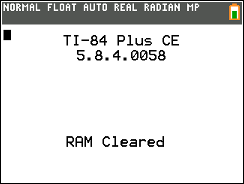
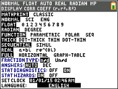
We’ll assume that you’re starting with a clean RAM. First of all enable Stat Diagnostics. You can find the flag in the mode menu.

Then head over to the list editor. You can reach it by pressing the stat key and then enter to select the first option (Edit)

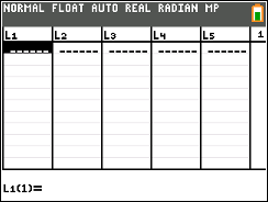
Once there you can input your data in L1 and L2 or two lists of your choice. It is common practice to put the x list in L1 and the y list in L2.

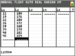
With the lists being defined you’re already able to run any function on them. Below is a list of the most common operations required.

---

2. Plot the data on a graph#

Now that you have the data in the lists you may want to plot a graph with the points. You may access the stat plot menu by pressing 2nd and y= in sequence. You can plot up to three series of data contemporarily. this is due to the limitation of having only six lists available to the user.

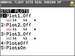
To plot your data, go to the slot you want to use (1,2,3).

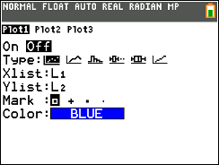
In this menu you can:

• Turn On/Off the plot
• Choose the style/type of the plot
• What list contains the x values
• What list contains the y values
• The style of the marks/points
• The color of the marks/points

Note that the above applies for the scatter type plot. Other types of plot may differ.

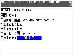
Turn on Plot 1.

Now go to the graph window by pressing graph.

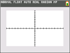
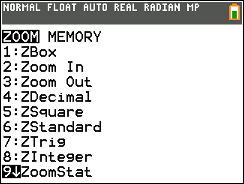
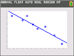
You now see that some of the points of your plot are not visible. To adjust the graph window to include all of your points, go to zoom -> 9 for ZoomStat.

Note that the stat plots may seem to behave differently than a function when traced with trace. This is especially true in an inverse correlation where the first point of the list might be graphed last. It may take a bit to get used to but my recommendation is to always keep a pointer on your table mentally.

---

3. Actually doing statistics#

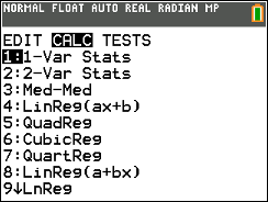
Now that the hard part is done it’s time to actually do shit with the numbers. The stat menu has a whole section dedicated to operations that can be done with the lists. To access it go to stat -> ->. From there you will usually use two submenus:

• 2-Var Stats to obtain the mean values and various other gimmicks
• Linreg(ax+b) to obtain data on the linear regression (r and the straight line)

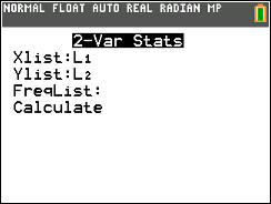
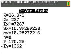
2-Var Stats#

This is the easiest menu to use, just put your x list and your y list and press calculate. The magic goblin inside your calculator does the rest!

The lion does not concern himself with FreqList

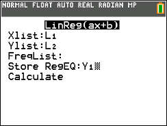
Linreg(ax+b)#

This is when shit starts to get real. First of all do not confuse this submenu with Linreg(a+bx), it does the same thing but outputs a and b inverted! Always look at where the x is to determine which is which!

To use this function you should input as usual the x and y lists, ignore the FreqList but pay attention to the Store RegEQ field. This field accepts an Y-Var as input and treats it like a pointer to store the produced equation. If you have no idea of what this means, please kys. Just know that you can put the Y= equation slot the produced line will be saved in. To access the variable, put your cursor on the Store RegEQ field and press vars -> -> -> enter and choose from the list the slot that the result will be saved in. This will overwrite any equation present in that slot! 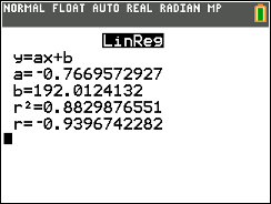Once you press calculate the a, b and r values will be shown. If you do not get r and r^2 make sure Stat Diagnostics is enabled in the mode menu

Conclusion#

This should answer all of your questions. If you still have questions please follow this guide.

— KMiguel